Central limit theorem
You can use the central limit theorem when sampling from a population that is not normally distributed.
Most of the time the population from which the samples are selected is not going to be normally distributed.
However, as the sample size increases, the sampling distribution of x̄ will approach a normal distribution.
Central limit theorem
For a large sample, usually when the sample is bigger or equal to 30, the sample distribution is approximately normal. This is true regardless of the shape of the population distribution.
The mean and standard deviation of the sampling distribution of x̄ are
- Keep in mind that the shape of the sampling distribution is not exactly normal, but approximately normal for a large sample size (n ≥ 30). As the sample size increases the approximation becomes more accurate.
- You can only use the central limit theorem when n ≥ 30 since the theorem applies to large samples only.
- Finally, in the formula for the standard deviation, n/N must be less than or equal to 0.05.
Example showing how to use the central limit theorem
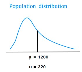
The mean mortgage paid by all householders in a large city is $1200 with a standard deviation of $320. The population distribution of mortgages for all householders in the city is skewed to the right. Find the mean and standard deviation of x̄ and describe the shape of its sampling distribution when the sample size is 64.
Solution
We see from the situation above that the population distribution is not normal since it is skewed to the right.
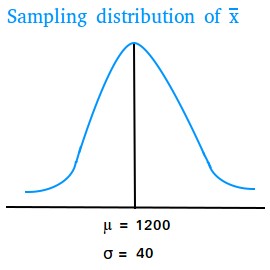
However, since the sample size is large (n ≥ 30), the shape of the sampling distribution is approximately normal.
Therefore, we can use the central limit theorem to infer the shape of the sampling distribution of x̄.
Let x̄ be the mean mortgage paid by a sample of 64 householders.
The mean of the sampling distribution of x̄ is:
| $$ {\mu_{\overline{x}} = \mu = 1200} $$ |
The standard deviation of the sampling distribution of x̄ is:
| $$ \sigma_{\overline{x}} = \frac{\sigma }{\sqrt{n} } $$ $$ \sigma_{\overline{x}} = \frac{320}{\sqrt{64} } $$ $$ \sigma_{\overline{x}} = \frac{320}{8 } $$ |
| $$ \sigma_{\overline{x}} = 40 $$ |
The figure below shows what the population distribution may look like.

The figure below shows what the sampling distribution of x̄ may look like.
