Construction of a frequency distribution

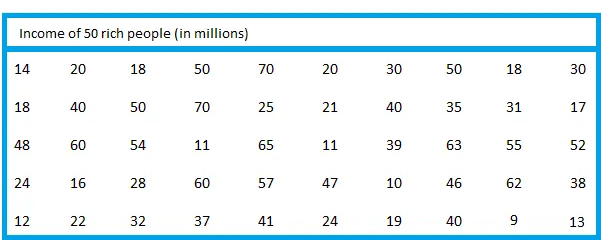
The construction of a frequency distribution table can be done using the procedure for constructing a frequency table and the quantitative raw data you see below.

Step 1:

Pick 6 as the number of classes.

Step 2: Use the class width formula to find the class width (See table below).

Round 10.166 down to 10 and use 10 as a convenient number for the class width.

Quantitative raw data

Step 3:

The lowest value in the list is 9. Let us use 9 as the lower limit of the first class.

To find the upper limit of the first class, subtract 1 from the class width and add the result to the lower limit of the first class.

10-1 = 9

9 + 9 = 18

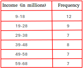
Therefore, the first class is 9-18

To find all the lower limits, just keep adding the class width to the previous lower limit.

Lower limits (in bold)

9 + 10 = 19

19 + 10 = 29

29 + 10 = 39

39 + 10 = 49

49 + 10 = 59

Upper limits (in bold)

To find all the upper limits, just keep adding the class width to the previous upper limit.

18 + 10 = 28

28 + 10 = 38

38 + 10 = 48

48 + 10 = 58

58 + 10 = 68

All you need to do now is to count the frequency of these classes. For example, to know the frequency of 19-28, just count all the numbers between 19 and 20, starting with 19 and ending with 28.

Notice that the sum of all the frequencies is equal to 50.

Construction of a frequency distribution, relative frequency and percentage distribution

The relative frequency and percentage can be found using the same formula we used in this lesson.

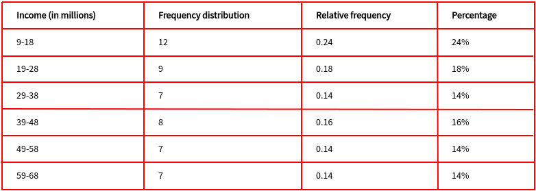
The relative frequency of 9 for instance is 9/50  = 0.18

To find the percentage, just multiply 0.18 by 100

0.18 × 100 = 18

The percentage is 18%

The table below shows the frequency distribution, the relative frequency, and the percentage distribution for the data set above.

Notice that the sum of all the relative frequencies is equal to 1 and the sum of all the percentages is equal to 100%