Continuous probability distribution

The continuous probability distribution is a table that shows the frequency and relative frequency of a continuous random variable. Recall that a continuous random variable can take any value over an interval or intervals. For example, suppose students have 60 minutes to finish a test. The time it takes students to finish the test can take any value over an interval such as an interval of 45 minutes to less than 46 minutes or [45, 46].

Suppose a math test is given to all 4000 students enrolled at a university. Suppose also that we have the following frequency and relative frequency distribution of "time it takes students to finish the test"

Time it takes students to complete a test (in minutes) or x	f	Relative frequency
45 to less than 46	80	0.02
46 to less than 47	200	0.05
47 to less than 48	600	0.15
48 to less than 49	1600	0.4
49 to less than 50	600	0.15
50 to less than 51	500	0.125
51 to less than 52	300	0.075
52 to less than 53	120	0.03
	N = 4000	Sum  = 1

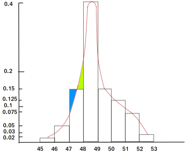
Below, we show a histogram and an approximation of the probability distribution curve of the continuous random variable x. The curve is also called probability density function. This is what the curve will approximately look like if you try to show the time it took the 4000 students (or population) to finish the test. This is not a perfect graph!

Some important observations about the continuous probability distribution

Did you notice the following characteristics about the continuous probability distribution?

a. The total probability of all the intervals which x can take on is equal to 1.

b. The area under the normal curve between 47 and 48 is shaped almost like a trapezoid. This area under the normal curve is the same as the area of the rectangle. This is so because the area of green rectangle is the same as the area of the blue rectangle.

Therefore, we can approximate the percentage of students who took 45 to less than 46 minutes to finish the test by looking for the area under the curve. In our example, it is not necessary since we can find that with the area of the rectangle.

Height of rectangle  = 0.15 and width = 1

Area = 0.15 times 1 = 0.15 = 15%

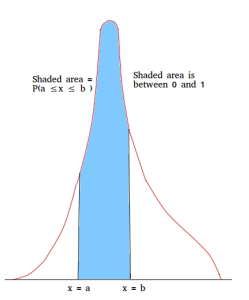
c. The area under the curve between any two points is between 0 and 1 and it is a measure of the probability between these two points as shown below.

d. The probability that a continuous random variable take on a single value is always equal to zero. This makes sense since a single value does not create an area.

Using our previous example P(x = 47) = 0. As you can see x = 47 is just a line, so there is no area and therefore no probability.

In general, if a and b are two of the values that x can take, then P(a) = 0 and P(b) = 0

We can then make the following conclusion.

For a continuous random variable, P(a ≤ x ≤ b) = P(a < x < b)