Sampling distribution

What is a sampling distribution? As stated in the previous lesson, the population mean is always constant. However, different samples of the same size drawn from the population will yield different values for the sample mean or x̄. 

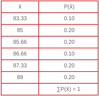
Consequently, the sample mean, x̄ , is a random variable and just like any other random variables, the sample mean x̄ has a probability distribution. This probability distribution of x̄ is called sampling distribution as shown in the table above.

How to find the sampling distribution of x̄ for a sample size of 3 using a population size of 5

In our previous lesson, the scores for 5 students were the followings:             

80         85          85          90             92

These 5 scores represent the entire population and population mean is 86.4. Suppose we draw 3 scores from the population to see what the average is going to be.

How many possible samples of 3 scores each can be selected without replacement from the population which has 5 elements?

We need to use the combination formula.

$$ {n \choose r} = {5 \choose 3} = \frac{5!}{3!(5-3)!} = \frac{5×4×3×2×1}{3!(2)!} $$
$$ {5 \choose 3} = \frac{5×4×3×2×1}{3×2×1(2×1)} = \frac{120}{12} = 10 $$

Let A =  80,      B  =  85      C  = 85,     D =  90,       E = 92

Below we list all the different samples.

ABC,  ABD,  ABE,  ACD,  ACE,  ADE,  BCD,  BCE,  BDE,  CDE

Scores in the sample are

80, 85, 85                     80, 85, 90

80, 85, 92                     80, 85, 90

80, 85, 92                     80, 90, 92

85, 85, 90                     85, 85, 92

85, 90, 92                     85, 90, 92

The table below shows all possible samples and their means

Scores in the sample	x̄
80, 85, 85	83.33
80, 85, 90	85
80, 85, 92	85.66
80, 85, 90	85
80, 85, 92	85.66
80, 90, 92	87.33
85, 85, 90	86.66
85, 85, 92	87.33
85, 90, 92	89
85, 90, 92	89

Now, we can create a table that shows the frequency and relative frequency distributions of x̄

x̄	f	Relative frequency
83.33	1	1/10 = 0.10
85	2	2/10 = 0.20
85.66	2	2/10 = 0.20
86.66	1	2/10 = 0.10
87.33	2	2/10 = 0.20
89	2	2/10 = 0.20

Finally, we show the sampling distribution of x̄ for a sample size of 3

x̄	P(x̄)
83.33	0.10
85	0.20
85.66	0.20
86.66	0.10
87.33	0.20
89	0.20
	∑P(x̄) = 1